In recent years, combining machine learning with traditional scientific computing has given rise to innovative approaches like Physics-Informed Neural Networks (PINNs). These neural networks are designed to directly incorporate the governing physical laws described by differential equations into the training process. This blog post explores the basics of PINNs using MATLAB, drawing on insights from Conor Daly’s deep dive session on implementing and training these neural networks.

What are Physics-Informed Neural Networks?

Physics-Informed Neural Networks (PINNs) are a class of neural networks that leverage physical laws, represented as differential equations, to guide their learning process. Unlike traditional neural networks that solely rely on data, PINNs integrate prior knowledge about the physical system, making them particularly useful in scenarios with limited data or complex physical phenomena.

The primary goal of PINNs is to ensure that the neural network's outputs satisfy the underlying physics of the problem. This is achieved by incorporating the differential equations directly into the training loss function, effectively guiding the network to learn solutions that adhere to the laws of physics.

Setting Up PINNs in MATLAB

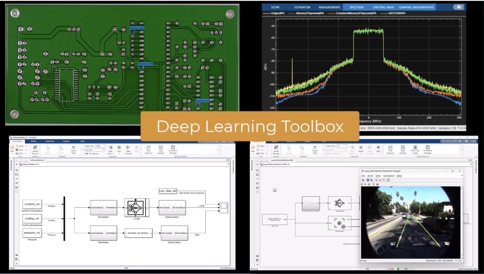
In our deep dive, we focused on developing a simple PINN to model a classic mass-spring-damper system, governed by a second-order ordinary differential equation. We highlighted how MATLAB’s Deep Learning Toolbox can be effectively utilised to build, train, and analyse PINNs.

1. Autodifferentiation in MATLAB: 

We emphasised the importance of autodifferentiation, which is available in MATLAB through the Deep Learning Toolbox. Autodifferentiation allows the calculation of gradients automatically, which is essential for training neural networks and implementing PINNs effectively. MATLAB’s support for reverse-mode autodifferentiation simplifies the process of computing the necessary derivatives during training.

2. Choosing the Example: Mass-Spring-Damper System: 

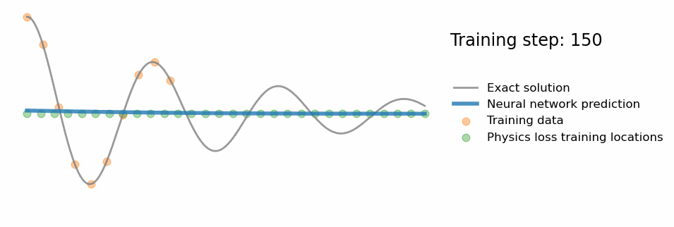
To introduce PINNs, Connor chose a classic mass-spring-damper system. This system is defined by a second-order differential equation representing the dynamics of a mass attached to a spring and damper. By using this example, we demonstrated how to apply PINNs to a well-understood physical system, making the learning process more relatable.

3. Setting Up the Neural Network:

The neural network setup in MATLAB involved defining the input and output sizes, the number of hidden units, and the types of layers used. We used a simple feedforward neural network with fully connected layers and hyperbolic tangent (tanh) activation functions. MATLAB’s syntax for developing neural network layers and combining them into a network was straightforward, making it easy to modify layer types and sizes to suit different problems.

Training the PINN

1. Defining the Loss Function

The loss function in PINNs typically includes two parts: a data loss and a physics-informed loss. The data loss corresponds to discrepancies between the network's predictions and actual observed data. In contrast, the physics-informed loss enforces the physical laws by minimising the residuals of the differential equations.

In the mass-spring-damper example, the physics-informed loss is calculated using the second derivative of displacement with respect to time. We showed how MATLAB’s `dlgradient` function can be used to compute these derivatives, leveraging the power of autodifferentiation.

2. Optimisation and Training Loop

The training process involves running an optimisation loop using the Adam optimiser. Connor demonstrated how to set up training parameters such as the learning rate and number of iterations. We also showed how to monitor training progress by plotting the loss values.

Extending PINNs to More Complex Systems

One insightful question raised was how to handle cases where no analytical solution is available for comparison. The PINN approach remains valuable even in such cases, as the physics-informed loss term is inherently unsupervised and does not require an analytical solution. This flexibility makes PINNs suitable for a wide range of applications, including those with complex, non-linear, or unknown dynamics.

Our deep dive into Physics-Informed Neural Networks with MATLAB provided a comprehensive overview of setting up, training, and analysing PINNs. By combining neural network learning with physical laws, PINNs offer a robust approach to solving differential equations, especially in cases with limited data or complex physical interactions. MATLAB's tools and capabilities streamline the implementation of PINNs, making it accessible for engineers and scientists looking to leverage the power of physics-informed machine learning.