“I do not fear computers. I fear the lack of them."
– Isaac Asimov
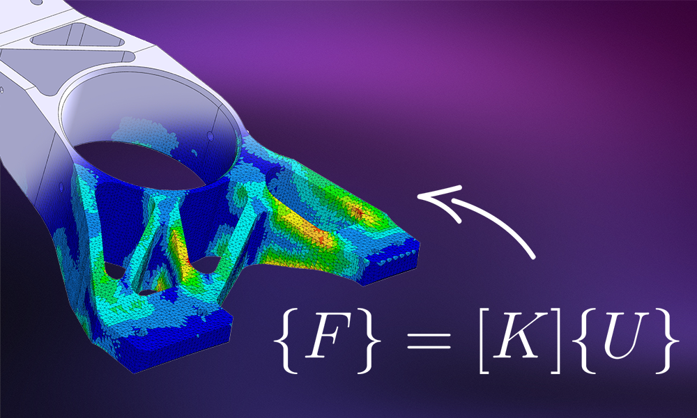
Motivation 🧠
If a component is to be calculated, it is generally possible to search the literature for corresponding closed-form solutions in order to describe the physical behaviour of a component by means of an equation.
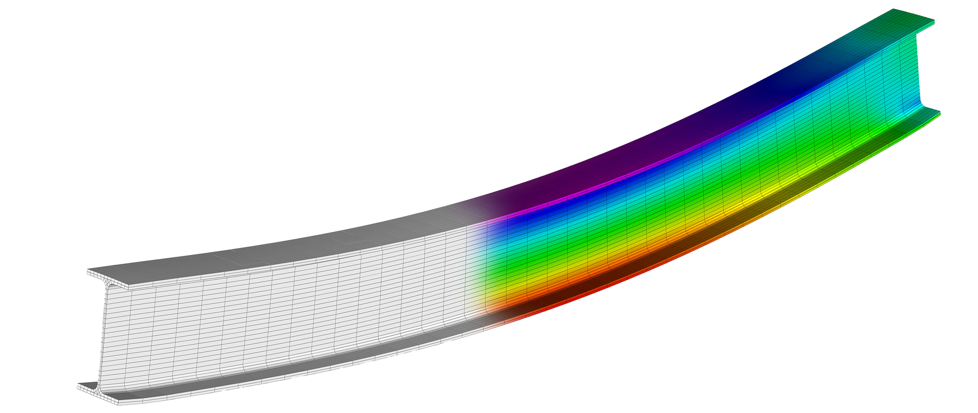
For example, we can use the following analytical solution for an I-beam to calculate the deflection:
\begin{equation} u = \frac{FL^3}{3EI} + \frac{ML^2}{2EI} \end{equation}
Where I is the "Second Moment of Area":
\begin{equation} I = \frac{1}{12}(BH^3 - bh^3) \end{equation}

As I mentioned in my "Beginner's Guide to FEM"...whenever engineers solve complex problems involving complex geometries, loading conditions or material laws, they cannot use classical analytical approaches using closed-form methods.
FEM offers a way to solve a problem where an analytical solution does not exist!
Introduction 👇
Whenever we cannot use the aforementioned approach, we have to talk about numerical methods such as the Finite Element Method (FEM) which discretises, or subdivides our domain into finite elements. We can call ourselves incredibly lucky that today's computer aided engineering (CAE) tools allow for automatic mesh generation and solving these systems. We do not have to waste engineering brain power anymore on deriving equations for new problems and start "from scratch", but can instead use FEA software tools that do the job for us.
We could technically derive the equations by simply taking the heat equation and deriving all equations from that one. From my experience teaching students, the easier approach is to describe the behaviour of a single bar element and model it as a spring. The behaviour of each element generally requires the development of partial differential equations (PDEs) for the problem and formulation of its weak form. PDEs...weak form...?
Don't worry. That's a bit of an advanced topic and will not be covered in this beginner friendly piece. We derive the basic equations without considering governing partial differential equations, weak forms or any other fancy methods.
We solely focus on deriving the equation for a single one-dimensional bar element which will be the basis to derive and solve bigger systems. The following approach will be used:
1. Look at force equilibrium of the element – assume that the sum of the nodal internal forces acting on the element is equal to zero
2. Apply Hooke’s law, which states that the stress \(\sigma\) is a linear function of the strain \(\epsilon\)
\begin{equation} \sigma = E \epsilon \end{equation}
3. Derive matrix for of the element stiffness matrix \(\mathbf{K}\) that relates the force and displacement matrices
4. ...Profit! 🚀
Notation ✍️
Nomenclature of Elements & Nodes 📝
When talking about the FEM, a simple notation will be used to denote element and node numbers.
- Element numbers are denoted by superscripts
- Node numbers are denoted by subscripts
When the variable is a vector with components in specific directions, the component is given after the number. In any other case we assume that we mean the global node number.
Example:
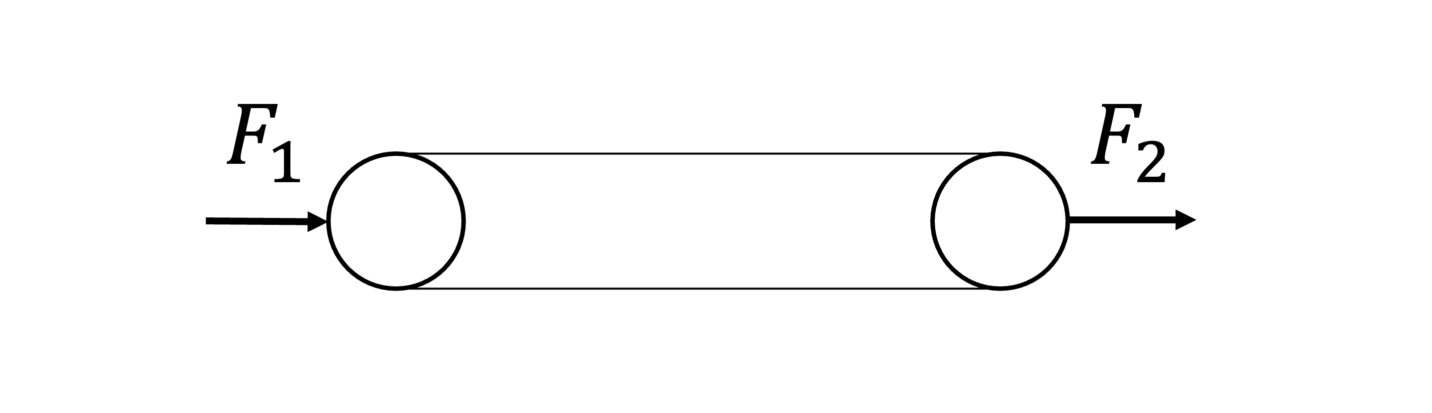
The image below shows a simple version of one bar element. The first node is on the left side, the second node on the right side, as indicated by the naming of the displacement u. The element is kept general in this case but will be renamed once we talk about bigger systems and need to distinguish between elements. It will also help you when we work on the "matrix assembly", so putting all matrices together to build a global matrix of all elements. Stay tuned!
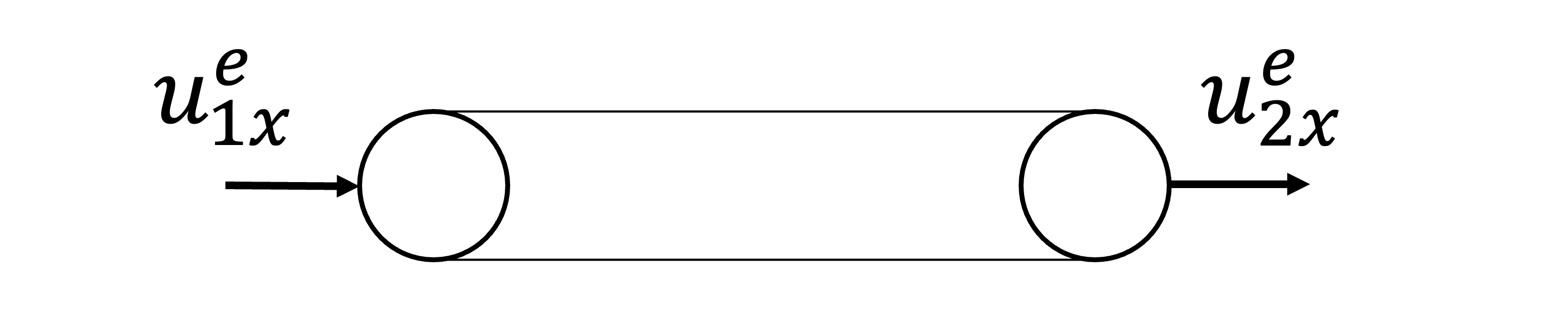
To reemphasise, for more complex cases where we have multiple elements in a system, \(u^2_{3x}\) would mean that we talk about the displacement of node 3 at element 2 in x direction – because multiple directions could be possible such as y, or if we talk about three dimensions, even z.
If that is not clear just yet, don't worry! You will understand it once we deal with bigger systems that we are going to solve! 🙂 It might seem annoying to do this but you will see that you understand the derivations much more easily if we do it in such a way.
The more familiar you become with the method, the less we will use this notation as it will "click" at some point and you'll become more proficient in using the method.
Force Convention 📄
We distinguish internal axial forces (and stresses) as well as nodal internal forces. The internal force is positive in tension and negative in compression, i.e. the force is positive when it points out from the surface on which it is acting and the nodal internal forces are positive when they point in the positive x-direction.
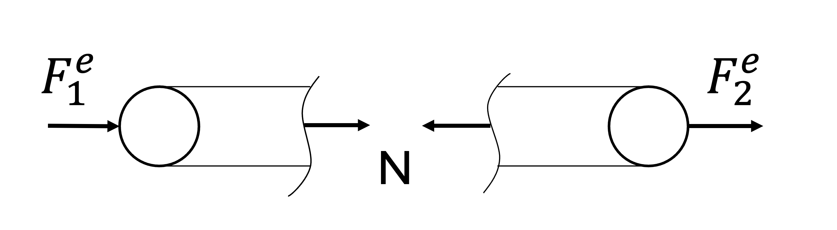
A Single Bar Element ☝️
We will model each of our homogeneous bar elements as a linear-elastic spring, subjected to Hooke's law \(F = KU\). We first note the correlation between normal Force \(N\) , the cross sectional area \(A\) and the uniaxial tensile stress \(\sigma\)
\begin{equation} \sigma = \frac{N}{A} \end{equation}
With Hooke’s law (\(\sigma = E \epsilon\)) and the one dimensional distortion
\begin{equation} \epsilon = \frac{du(x)}{dx} = \frac{\Delta l^e}{l^e_0} \end{equation}
follows that with the length variation \(\Delta l^e\) and the original length of the bar \(l^e_0\) and rearranging equation 2
\begin{equation} N = A \sigma = AE \epsilon = AE \frac{\Delta l^e}{l^e_0} \end{equation}
or rewrite it simply to
\begin{equation} N = \frac{EA}{l^e_0} \Delta l^e \end{equation}
which finally gives us
\begin{equation} N = k^e \Delta l^e \end{equation}
We call \(k^e\) the element stiffness (sometimes called extensional stiffness) – the superscript e indicates that we refer to one single element only. The elongation \(\Delta l^e\) can be described as a function of displacements of the nodes of a bar
\begin{equation} \Delta l^e = u^ e_2 - u^ e_1 \end{equation}
If we apply the equilibrium condition on the bar, i.e. we take the sum of the forces applied on each node of the element and say they are equal to zero
\begin{equation} F_1 + F_2 = 0 \end{equation}
We now apply the same principle to the other free body diagram.

What happens if we evaluate the equilibrium?
The left side gives us
\begin{equation} F^e_1 + N = 0 \end{equation}
or
\begin{equation} F^e_1 = -N \end{equation}
We do the same for the right side
\begin{equation} F^e_2 - N = 0 \end{equation}
yielding \(F^e_2 = N\) as N for the right side shows to the left, so is accounted for negative!
Bringing Everything Together 📖
Let's now use everything we have so far.
\begin{equation} F^e_2 = N = k^e \Delta l^e = k^e (u^ e_2 - u^ e_1 ) = k^e u^ e_2 - k^e u^ e_1 \end{equation}
We do not have to do the same for \(F^e_1 \) as we know from equation 10 that
\begin{equation} F^e_1 = -F^e_2 \end{equation}
The force equilibrium in matrix notation (tensor notation) looks as follows
\begin{equation} \underline{F}^e = \begin{bmatrix} F^e_1 \\ F^e_2 \\ \end{bmatrix} = \begin{bmatrix} -N \\ N \\ \end{bmatrix} = k^e \begin{bmatrix} 1 & -1 \\ -1 & 1 \\ \end{bmatrix} \begin{bmatrix} u^e_1 \\ u^e_2 \\ \end{bmatrix} = \underline{\underline{K}}^e \underline{d}^e \end{equation}
The matrix \(\underline{\underline{K}}^e\) is called the element stiffness matrix. From a mathematical point of view, this matrix is positive semi-definite which is symmetric with non-negative eigenvalues.
The vector \(\underline{\underline{d}}^e\) is called the element displacement matrix and \(\underline{\underline{F}}^e\) the element force matrix.
The stiffness matrix establishes the correlation between nodal displacements and nodal forces. Keep in mind that the matrix \(\underline{\underline{K}}^e\) is always singular which means the matrix is non-invertible and its determinant is zero.
To physically interpret the matrix singularity, imagine that our little bar is able to undergo rigid body motions and flow around in the universe as it is not fixed yet. Or to formulate this more physically: We have not added boundary conditions yet!
To see that this is the case, you can simple add the rows of the stiffness matrix and you will see that the equations are linearly dependent. When does this happen? Whenever our system is statically under-determined!
The mathematical property of the matrix being positive semi-definite follows from the non-negativity of the deformation energy of our bar for arbitrary nodal displacements \(\underline{\underline{d}}^e\) (We have always mechanical input in our system. No matter if it is tension or compression!)
\begin{equation} W^e \left(\underline{d}^e \right) = \frac{1}{2} \left(\underline{d}^e \right)^\top \underline{\underline{K}}^e \underline{d}^e \geq 0 \end{equation}
Don't worry. We will not need this equation. I simply wanted to put the equation here for completion and in case you want to look it up online...and also because I seek external validation and think "complex" equations are cool.
To summarise, here's a simplified version of the formula we derived in matrix notation.
\begin{equation} \begin{bmatrix} K & -K \\ -K & K \\ \end{bmatrix} \begin{bmatrix} U_1 \\ U_2 \\ \end{bmatrix} = \begin{bmatrix} F_1 \\ F_2 \\ \end{bmatrix} \end{equation}
If we write the same equation in the form of a symbolic representation, we receive the renowned "FEA Formula".
\begin{equation} \mathbf{KU} = \mathbf{F} \end{equation}
👉 In the next blog, we will have a look at a simple arithmetic example and cover how we can add boundary conditions to statically under-determined systems.
If this post was helpful to you, consider subscribing to receive the latest blogs, tutorials, code snippets and course updates! 🙂
And if you would love to see another topic on FEA, please leave a comment!👇
Keep engineering your mind! ❤️
Jousef